Kaggle Competition: Digit recognition on MNIST data
7/7/2017 Wei-Ying Wang
This is my tutorial about how to use Keras to construct a CNN model for digit recognition. The tutorial tried to be comprehensive about building CNN with Keras. Keras is designed to be easy to use and manipulate, however I found difficult to understand the structure I built when I first used it. I hope this tutorial can help smooth the learning curve of using Keras.
Most of the information is on chapter 2 and 3. I will emphasize a lot on knowing the number of parameters, inputs, and outputs.
To use this Ipython notebook, please download the data train.csv and test.csv from Kaggle Digit Recognizer webpage, and put it into the right directory.
I eventually got 99.21% correction rate. Note that MNIST dataset is famous online, and it is not surprising that one can get 100% on the test set provided by Kaggle, since it is not difficult to find all the MNIST data somewhere else. The real winner (correct me if I am wrong) so far is from Dan Cireşan et. al. 2012, who got 99.77% correction rate, which achieved near human performance. He used CNN, too.
Table of content
1. Import modules and preprocessing the data
2. A Typical CNN structure: one CNN layer
3. Stack more CNN layers
4. Using the learned trained model to predict the test set
You can download this Ipython notebook at My Github Website.
1. Import modules and preprocessing the data
from importlib import reload

from __future__ import print_function
import keras
import numpy as np
import matplotlib.pyplot as plt
from keras.models import Sequential
from keras.layers import Dense, Dropout,Flatten,Conv2D, MaxPooling2D
from keras.optimizers import RMSprop
from keras.utils.np_utils import to_categorical
#from keras.preprocessing.image import ImageDataGenerator
import pandas as pd
from sklearn.model_selection import train_test_split
import Aux_fcn
reload(Aux_fcn)
Using TensorFlow backend.


<module 'Aux_fcn' from 'D:\\Dropbox\\Job finding\\Some machine learning topic\\code\\MNIST_Kaggle\\github\\Aux_fcn.py'>
Import the data ( Download at https://www.kaggle.com/c/digit-recognizer/data), and be sure to put it into the right place.
train = pd.read_csv('../data/train.csv')
test  = pd.read_csv('../data/test.csv')
train.head()
| label | pixel0 | pixel1 | pixel2 | pixel3 | pixel4 | pixel5 | pixel6 | pixel7 | pixel8 | ... | pixel774 | pixel775 | pixel776 | pixel777 | pixel778 | pixel779 | pixel780 | pixel781 | pixel782 | pixel783 | |
|---|---|---|---|---|---|---|---|---|---|---|---|---|---|---|---|---|---|---|---|---|---|
| 0 | 1 | 0 | 0 | 0 | 0 | 0 | 0 | 0 | 0 | 0 | ... | 0 | 0 | 0 | 0 | 0 | 0 | 0 | 0 | 0 | 0 |
| 1 | 0 | 0 | 0 | 0 | 0 | 0 | 0 | 0 | 0 | 0 | ... | 0 | 0 | 0 | 0 | 0 | 0 | 0 | 0 | 0 | 0 |
| 2 | 1 | 0 | 0 | 0 | 0 | 0 | 0 | 0 | 0 | 0 | ... | 0 | 0 | 0 | 0 | 0 | 0 | 0 | 0 | 0 | 0 |
| 3 | 4 | 0 | 0 | 0 | 0 | 0 | 0 | 0 | 0 | 0 | ... | 0 | 0 | 0 | 0 | 0 | 0 | 0 | 0 | 0 | 0 |
| 4 | 0 | 0 | 0 | 0 | 0 | 0 | 0 | 0 | 0 | 0 | ... | 0 | 0 | 0 | 0 | 0 | 0 | 0 | 0 | 0 | 0 |
5 rows × 785 columns
test.head()
| pixel0 | pixel1 | pixel2 | pixel3 | pixel4 | pixel5 | pixel6 | pixel7 | pixel8 | pixel9 | ... | pixel774 | pixel775 | pixel776 | pixel777 | pixel778 | pixel779 | pixel780 | pixel781 | pixel782 | pixel783 | |
|---|---|---|---|---|---|---|---|---|---|---|---|---|---|---|---|---|---|---|---|---|---|
| 0 | 0 | 0 | 0 | 0 | 0 | 0 | 0 | 0 | 0 | 0 | ... | 0 | 0 | 0 | 0 | 0 | 0 | 0 | 0 | 0 | 0 |
| 1 | 0 | 0 | 0 | 0 | 0 | 0 | 0 | 0 | 0 | 0 | ... | 0 | 0 | 0 | 0 | 0 | 0 | 0 | 0 | 0 | 0 |
| 2 | 0 | 0 | 0 | 0 | 0 | 0 | 0 | 0 | 0 | 0 | ... | 0 | 0 | 0 | 0 | 0 | 0 | 0 | 0 | 0 | 0 |
| 3 | 0 | 0 | 0 | 0 | 0 | 0 | 0 | 0 | 0 | 0 | ... | 0 | 0 | 0 | 0 | 0 | 0 | 0 | 0 | 0 | 0 |
| 4 | 0 | 0 | 0 | 0 | 0 | 0 | 0 | 0 | 0 | 0 | ... | 0 | 0 | 0 | 0 | 0 | 0 | 0 | 0 | 0 | 0 |
5 rows × 784 columns
print('training data is (%d, %d) and test data is (%d, %d).'% (train.shape+test.shape))
training data is (42000, 785) and test data is (28000, 784)
#%%
X_train_all = (train.ix[:,1:].values).astype('float32')/255 # all pixel values, convert to value in [0,1]
y_train_all = train.ix[:,0].values.astype('int32') # only labels i.e targets digits
y_train_all= to_categorical(y_train_all) # This convert y into onehot representation
X_test = (test.values).astype('float32')/255 # all pixel values
X_train, X_val, y_train, y_val = train_test_split(X_train_all, y_train_all, test_size=0.10, random_state=42)
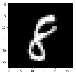
We have to map the image vectors (size 784) back to image. Specially, we have to convert to (28,28,1), since the convolution layer of Kares only accept image of dimension 3 (the last dim is the color channel).
X_train_img=np.reshape(X_train,(X_train.shape[0],28,28,1))
X_test_img = np.reshape(X_test,(X_test.shape[0],28,28,1))
X_val_img = np.reshape(X_val,(X_val.shape[0],28,28,1))
plt.imshow(X_train_img[0,:,:,0],cmap = 'gray')
plt.show()
---------------------------------------------------------------------------

TypeError                                 Traceback (most recent call last)

<ipython-input-5-9ad6acbe2367> in <module>()
      1 plt.imshow(X_train_img[0,:,:,0],cmap = 'gray')
      2 plt.show()
----> 3 plt.imsave('one_training_sample.png')


C:\WinPython-64bit-3.6.0.1Qt5\python-3.6.0.amd64\lib\site-packages\matplotlib\pyplot.py in imsave(*args, **kwargs)
   2318 @docstring.copy_dedent(_imsave)
   2319 def imsave(*args, **kwargs):
-> 2320     return _imsave(*args, **kwargs)
   2321
   2322


TypeError: imsave() missing 1 required positional argument: 'arr'
2. A Typical CNN structure: one CNN layer.
-
The original input image is $28\times28$, so the
input_shape=(28,28,1), where1indicates that number of color channels is 1. -
In the following convolution layer, there are 32 filters, and each filters is $3\times3$.
- You can set border differently by:
border_mode='same', 'fall', or 'valid' (default) - With
validborder, after convolution (with stride=0), the filted image size is(28-2)x(28-2) = 26x26
- You can set border differently by:
- Set stride 2 by
subsample=(2,2). Note that stride affect before applying filter. So now the filtered and subsampled image is $13 \times 13$
- There are $32\cdot3\cdot3+32 =320$ parameters.
- Each “pixel” of the filted (and subsampled) image is obatained by $\sum_{i=1}^9 w_i x_i +b$, where $w_1,…,w_9,b\in \mathbb{R}^{10}$ are parameters and $(x_1,…,x_9)$ is a $3\times3$ image patches in the original input image.
-
Using
reluunits byactivation='relu', then max Pooling by 2. So the output of this CNN layer will be $32$ of $6\times 6$ “images”. -
If the next layer is ‘softmax’, one has to ‘flatten’ the output of the CNN layer. After flatten, the input of the next layer is of $6\cdot 6\cdot 32=1152$ values.
- So the last layer (‘softmax’) would require $1152\cdot 10+10$ parameters.
model = Sequential()
model.add(Conv2D(32, 3, 3,
                 activation='relu',subsample=(2,2),
                 input_shape=(28,28,1)))
model.add(MaxPooling2D(pool_size=(2, 2)))
model.add(Flatten(name='flatten'))
model.add(Dense(10, activation='softmax'))
model.summary()
____________________________________________________________________________________________________
Layer (type)                     Output Shape          Param #     Connected to
====================================================================================================
convolution2d_1 (Convolution2D)  (None, 13, 13, 32)    320         convolution2d_input_1[0][0]
____________________________________________________________________________________________________
maxpooling2d_1 (MaxPooling2D)    (None, 6, 6, 32)      0           convolution2d_1[0][0]
____________________________________________________________________________________________________
flatten (Flatten)                (None, 1152)          0           maxpooling2d_1[0][0]
____________________________________________________________________________________________________
dense_1 (Dense)                  (None, 10)            11530       flatten[0][0]
====================================================================================================
Total params: 11,850
Trainable params: 11,850
Non-trainable params: 0
____________________________________________________________________________________________________
Before fitting the parameters, we need to compile the model first.
model.compile(loss='categorical_crossentropy',
              optimizer='RMSprop',
              metrics=['accuracy'])
We can now fit the parameters. Note that:
- A better
batch_sizeshould be the exponent of 2, this is from the document of Keras. - Each epoch will scan through all the training data. Where each update of parameters uses
batch_sizeof data (It will be chosen randomly through each epoch.) initial_epochallows you to continuoue your last parameter fitting.- verbose controls the infromation to be displayed. 0: no information displayed, 1: max infomation, 2: somewhat between.
batch_size = 64
epochs = 20
history = model.fit(X_train_img, y_train,
                    batch_size=batch_size,
                    nb_epoch=epochs,
                    verbose=2,
                    validation_data=(X_val_img, y_val),
                    initial_epoch=10)
Train on 37800 samples, validate on 4200 samples
Epoch 11/20
3s - loss: 0.0478 - acc: 0.9864 - val_loss: 0.0749 - val_acc: 0.9764
Epoch 12/20
3s - loss: 0.0464 - acc: 0.9865 - val_loss: 0.0753 - val_acc: 0.9764
Epoch 13/20
3s - loss: 0.0453 - acc: 0.9872 - val_loss: 0.0741 - val_acc: 0.9769
Epoch 14/20
3s - loss: 0.0440 - acc: 0.9876 - val_loss: 0.0754 - val_acc: 0.9762
Epoch 15/20
3s - loss: 0.0431 - acc: 0.9880 - val_loss: 0.0731 - val_acc: 0.9769
Epoch 16/20
3s - loss: 0.0418 - acc: 0.9880 - val_loss: 0.0730 - val_acc: 0.9748
Epoch 17/20
3s - loss: 0.0413 - acc: 0.9888 - val_loss: 0.0766 - val_acc: 0.9755
Epoch 18/20
3s - loss: 0.0398 - acc: 0.9888 - val_loss: 0.0767 - val_acc: 0.9769
Epoch 19/20
3s - loss: 0.0394 - acc: 0.9891 - val_loss: 0.0763 - val_acc: 0.9779
Epoch 20/20
3s - loss: 0.0384 - acc: 0.9892 - val_loss: 0.0759 - val_acc: 0.9764
We can see that after 20 epoch, the validation accuracy is not improved (around 97.6%). The training set accuracy is about 98.8%. We should first try more complicated model to see if the training set accuracy get higher.
3. Stack more CNN layers
In the following model, we have:
1. First CNN layer:
- The input is $28\times 28$
- Filter (kernel) size: $5\times 5$. With
validpadding. - Number of filters: 64.
- The output is 64 of $24\times 24$ filted images. i.e. $ 24\times 24\times 64$
- The number of parameters: $25\cdot 64+64=1664$.
2. Second CNN layer:
- The input is $ 24\times 24\times 64$
- Filter (kernel) size: $3\times 3 \times 64$. With
validpadding.- This might concern you a lot… is it resonable? The convolution aggregate through all the images of previous layer. A better design of this layer is to use more (or equal number) of filters (instead of 32, as I put here) than 64. I put 32 just for demonstration.
- Number of filters: 32.
- The output is 32 of $22\times 22$ filted images. i.e. $22\times 22\times 32$
- The number of parameters: $3\cdot 3 \cdot 64\cdot 32+32 = 18464$.
- Think this way: There are 64 nodes, and each node is $24\times 24$ filted images.
3. Third: MaxPool layer:
- The output is $11\times 11\times 32$
4. Forth: A normal nural network layer with 128 nodes
- Each node here will connect to 32 nodes of previous layer. (Each node in previous layer is represented as a $11\times 11$ image.)
- The output is $11\times 11\times 128$.
- The number of parameters: $32\cdot 128+128=4224$
- Apply dropout rate 0.2 to prevent overfitting.
5. Fifth: Flatten the output of the previous layer:
- The output is $11\cdot 11\cdot 128=15488$ nodes
6. Final: 10 softmax units.
- The number of parameter: $15488*10+10=154898$
model = Sequential()
model.add(Conv2D(64, 5, 5,
                 activation='relu',
                 input_shape=(28,28,1)))
model.add(Conv2D(32, 3, 3, activation='relu'))
model.add(MaxPooling2D(pool_size=(2, 2)))
model.add(Dense(128, activation='relu'))
model.add(Dropout(0.2))
model.add(Flatten(name='flatten'))
model.add(Dense(10, activation='softmax'))
model.summary()
model.compile(loss='categorical_crossentropy',
              optimizer='RMSprop',
              metrics=['accuracy'])
____________________________________________________________________________________________________
Layer (type)                     Output Shape          Param #     Connected to
====================================================================================================
convolution2d_12 (Convolution2D) (None, 24, 24, 64)    1664        convolution2d_input_7[0][0]
____________________________________________________________________________________________________
convolution2d_13 (Convolution2D) (None, 22, 22, 32)    18464       convolution2d_12[0][0]
____________________________________________________________________________________________________
maxpooling2d_7 (MaxPooling2D)    (None, 11, 11, 32)    0           convolution2d_13[0][0]
____________________________________________________________________________________________________
dense_12 (Dense)                 (None, 11, 11, 128)   4224        maxpooling2d_7[0][0]
____________________________________________________________________________________________________
dropout_6 (Dropout)              (None, 11, 11, 128)   0           dense_12[0][0]
____________________________________________________________________________________________________
flatten (Flatten)                (None, 15488)         0           dropout_6[0][0]
____________________________________________________________________________________________________
dense_13 (Dense)                 (None, 10)            154890      flatten[0][0]
====================================================================================================
Total params: 179,242
Trainable params: 179,242
Non-trainable params: 0
____________________________________________________________________________________________________
batch_size = 64
epochs = 5
history = model.fit(X_train_img, y_train,
                    batch_size=batch_size,
                    nb_epoch=epochs,
                    verbose=2, # verbose controls the infromation to be displayed. 0: no information displayed
                    validation_data=(X_val_img, y_val),
                    initial_epoch=0)
Train on 37800 samples, validate on 4200 samples
Epoch 1/5
104s - loss: 0.1609 - acc: 0.9504 - val_loss: 0.0661 - val_acc: 0.9793
Epoch 2/5
104s - loss: 0.0577 - acc: 0.9828 - val_loss: 0.0519 - val_acc: 0.9848
Epoch 3/5
104s - loss: 0.0435 - acc: 0.9867 - val_loss: 0.0411 - val_acc: 0.9883
Epoch 4/5
104s - loss: 0.0370 - acc: 0.9884 - val_loss: 0.0497 - val_acc: 0.9848
Epoch 5/5
105s - loss: 0.0317 - acc: 0.9902 - val_loss: 0.0411 - val_acc: 0.9867
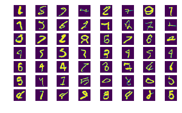
The following function shows the wrongly predicted images. Many of them I can’t even tell what it is…
Aux_fcn.plot_difficult_samples(model,X_val_img,y_val,verbose=False)
plt.show()
4200/4200 [==============================] - 4s
There are 56 wrongly predicted images out of 4200 validation samples
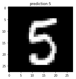
4. Using the learned trained model to predict the test set.
pred_classes = model.predict_classes(X_test_img)
28000/28000 [==============================] - 30s - ETA: 20s - ETA: 2s
i=10
plt.imshow(X_test_img[i,:,:,0],cmap='gray')
plt.title('prediction:%d'%pred_classes[i])
plt.show()
Appendix:
The function Aux_fcn.plot_difficult_samples is the following:
def plot_difficult_samples(model,x,y, verbose=True):
    """
    x: size(n,h,w,c)
    y: is categorical, i.e. onehot, size(n,p)
    """
    #%%

    pred_classes = model.predict_classes(x)
    y_val_classes = np.argmax(y, axis=1)
    er_id = np.nonzero(pred_classes!=y_val_classes)[0]
    #%%
    K = np.ceil(np.sqrt(len(er_id)))
    fig = plt.figure()
    print('There are %d wrongly predicted images out of %d validation samples'%(len(er_id),x.shape[0]))
    for i in range(len(er_id)):
        ax = fig.add_subplot(K,K,i+1)
        k = er_id[i]
        ax.imshow(x[er_id[i],:,:,0])
        ax.axis('off')
        if verbose:
            ax.set_title('%d as %d'%(y_val_classes[k],pred_classes[k]))